
Let’s discuss what linear regression is and how to use it. We will also use R to implement a linear regression model to a test dataset.
I assume that if you are reading this, you have a basic grasp of descriptive statistics (mean, median, mode, etc.). In other words, this is beginner-friendly!
And we will only go over the intuition: we will keep the mathematical formulas to a minimum 😉
If you want to learn how to use this model in R, I invite you you watch the following Youtube video, where I show you how to do this!
You can find the code for this video in this repo: https://github.com/alejandro-ao/ecommerce-project-r
What is linear regression?#
Linear Regression is a method we use in mathematics to find patterns in data. It’s far from being the most accurate method we have, but it’s very useful if some variables of your data are correlated.
For example, let’s say that you have a variable for the exam scores for a set of students. And you also have the number of hours they spent studying. If you plot scores against hours of study, you see that they seem correlated. As the hours of study increase, the score also seems to increase.
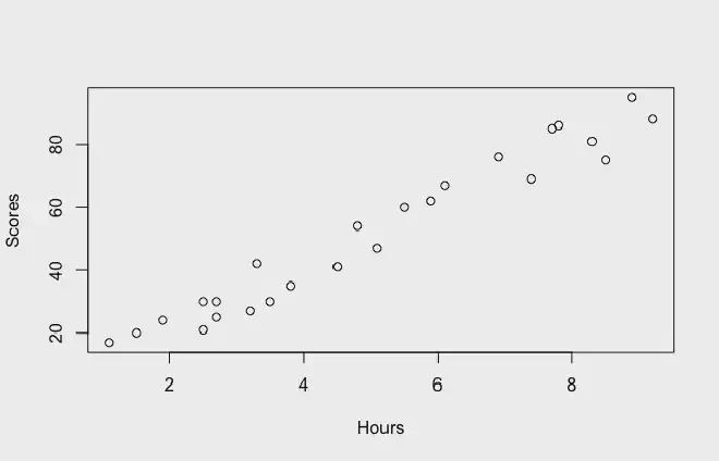
Once you find that your data seems to be correlated, you can fit a linear regression model to try to predict the score of any student based on the time they spent studying!
So you draw a line across all the points trying to make it as close to every single point as possible. This line is called the “regression line”.
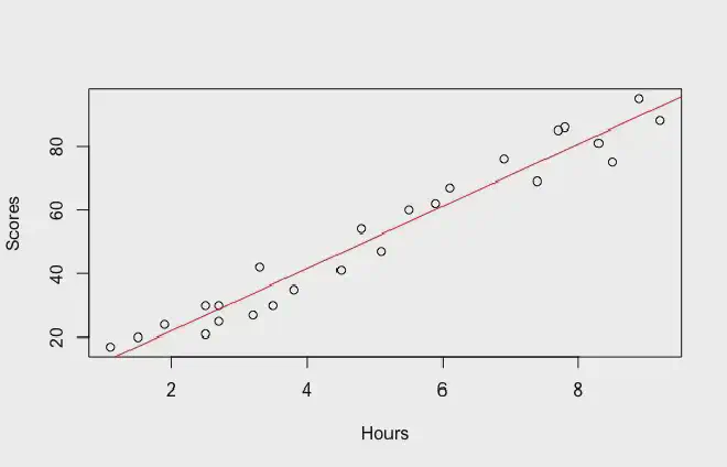
How to draw a regression line? As mentioned before, a regression line is a line that you draw over a set of points. This line is as close to every single point as possible. But what does that mean?
This means that we first need to draw a random line on top of our scatter plot. And we measure the distance from the line to every single point. We square each of those distances and then add them together. This number is called the sum of squares.
We then tilt the line a little and measure the sum of squares again.
In the end, after doing this many times, the regression line is the one with the smallest sum of squares. This will be the line that is as close to every point as possible.
How does the model work?#
Visually, all we are doing is drawing the regression line and then using it to predict the value of our variable at any given point.
As you might notice, the model is extremely inaccurate! It predicts that all the values fall on the regression line. But in reality, they are scattered around it!
Nevertheless, the regression line remains a very good descriptor of your data and its trend. Even if its predictions are not always very accurate, it is still a very good way to see how your data behaves.
And sometimes, the linear regression will actually be a good predictor. But only when the data is not very scattered. In other words, when all the points are closer to the line.
Here is another example of a linear regression where the data is not exactly close to the regression line. It plots the amount of money a client spends on an e-commerce platform per year against the Length of their membership.
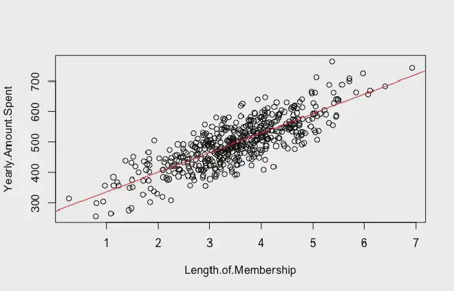
You can see that the data is correlated, but the average distance between the regression line and the dots is way larger than in our previous example.
Here, we find again the use of the sum of squares measure. It basically tells us how dispersed our data is. The bigger the sum of squares, the more dispersed the data. And thus, the least accurate our model will be.
The algebraic representation#
Of course, so far we have talked about the graphical interpretation. But we can also express the same thing with an algebraic expression. Here is where some formulas come up, so buckle up.
Every line on the plane has an equation that describes it in terms of f(x). To fit a linear regression model is to find the equation of the regression line. This way, it will be able to find an equation that looks like this:
where:
- is the predicted value for the response variable
- is the value of the predictor variable (hours of study in our previous example).
- are the coefficients that we need to find in order to actually draw the regression line. These are also approximations, that’s why we add a “^”.
So as you can see, can you tell what is the most important part of the work of fitting a linear regression model to a dataset? Right, it’s finding these linear coefficients that describe your regression line.
These are the coefficients that computer programs throw at you when you want to fit a linear regression to it.
Multivariable linear regression#
Of course, this is a very basic example. This kind of analysis happens very rarely in real life. More often than not, you have more than a single variable having an influence on your response variable.
So in reality, your linear model would look something like this:
where:
- is the predicted value for the response variable
- are the predictor variables
- are the coefficients of the model
So in a more realistic scenario, the previous example where we want to predict the test score of a student is better illustrated by a multilinear model like this one.
In this model, the other predictors represent things like “hours of sleep before the test”, “proximity to test location”, “hours of attendance to course”, etc.
As you might imagine, this model represents reality more accurately and it predicts the scores of a student. All because it takes more factors into account.
Conclusion#
Linear regression is one of the most common statistical learning models. Even though it is not the most accurate model, it is very used in the industry. Especially when you have many predictor variables that can help you make your model more accurate.